Kinematics

Overview

Kinematics is the study of motion without considering the forces causing the motion. It focuses on describing how position, velocity and acceleration change with time.

This topic forms the foundation for later chapters such as Forces, Dynamics, Circular Motion and Projectile Motion.

Kinematics can be approached through three connected languages:

• Words - describe the motion physically
• Graphs - visualise how quantities vary with time
• Equations - calculate unknown quantities

---

Core Ideas

Core Quantities in Motion

Scalars and Vectors

Scalars have magnitude only:

• distance
• speed
• time

Vectors have magnitude and direction:

• displacement
• velocity
• acceleration

See Vectors.

Distance and Displacement

Distance = total path length travelled.

• scalar
• always non-negative

Displacement = change in position from initial point to final point.

$$\vec{s}={\vec{r}}_{\text{final}}-{\vec{r}}_{\text{initial}}$$

• vector (see Vectors))
• in 1D, a vector can be represented with a signed scalar
• a signed scalar in 1D may be positive, negative, or zero

Example: Walk 3 m east then 3 m west.

• distance = 6 m
• displacement = 0 m

Speed and Velocity

Average speed

$$\text{average speed}=\frac{\text{total distance}}{\Delta t}$$

Average velocity

$$\text{average velocity}=\frac{\text{displacement}}{\Delta t},{\vec{v}}_{\text{avg}}=\frac{\Delta \vec{s}}{\Delta t}$$

Instantaneous velocity

$$\vec{v}=\frac{d\vec{s}}{dt}$$

Velocity includes direction. A negative velocity means motion in the chosen negative direction.

Acceleration

Acceleration is the rate of change of velocity:

$$\vec{a}=\frac{d\vec{v}}{dt}$$

It is a vector quantity.

• In 1D, positive acceleration does not always mean speeding up
• In 1D, negative acceleration does not always mean slowing down

In 1D, Whether speed increases depends on the relative directions of $v$ and $a$.

Velocity	Acceleration	Effect
+	+	speeds up
+	-	slows down
-	-	speeds up
-	+	slows down

For more detail: Kinematic Quantities and Sign Conventions

Sign Conventions (1D Motion)

A vector can be written as:

$$\vec{r}=|\vec{r}|\hat{u}$$

where $|\vec{r}|$ is the magnitude and $\hat{u}$ is a unit vector indicating direction.

For motion in one dimension, we first choose a positive reference direction, for example east along the $x$-axis, represented by $\hat{x}$.

A vector pointing in the positive direction is:

$$\vec{r}=|\vec{r}|\hat{x}$$

A vector pointing in the opposite direction is:

$$\vec{r}=|\vec{r}|(-\hat{x})=-|\vec{r}|\hat{x}$$

Hence, in 1D, direction can be represented simply by the sign of a scalar quantity:

• Positive sign: same direction as the chosen reference direction
• Negative sign: opposite direction to the chosen reference direction

Therefore, once a reference direction is chosen, a 1D vector can be represented by a signed scalar, where the magnitude gives size and the sign gives direction.

Example for vertical motion with upward positive, the signed scalar for the acceleration is:

$$a=-g$$

where $g=9.81{\text{m s}}^{-2}$ is the magnitude.

Average vs Instantaneous Quantities

Average values describe motion over an interval.

Instantaneous values describe motion at one moment.

Examples:

$${\vec{v}}_{\text{avg}}=\frac{\Delta \vec{s}}{\Delta t}$$ $$\vec{v}=\frac{d\vec{s}}{dt}$$ $$\vec{a}=\frac{d\vec{v}}{dt}$$

Motion Graphs Overview

Graphs are heavily tested in H2 Physics.

Displacement-Time Graph in 1D

Gradient gives velocity (signed scalar):

$$\text{gradient}=\frac{ds}{dt}=v$$

• positive slope → moving in positive direction
• zero slope → stationary
• steeper slope → larger speed

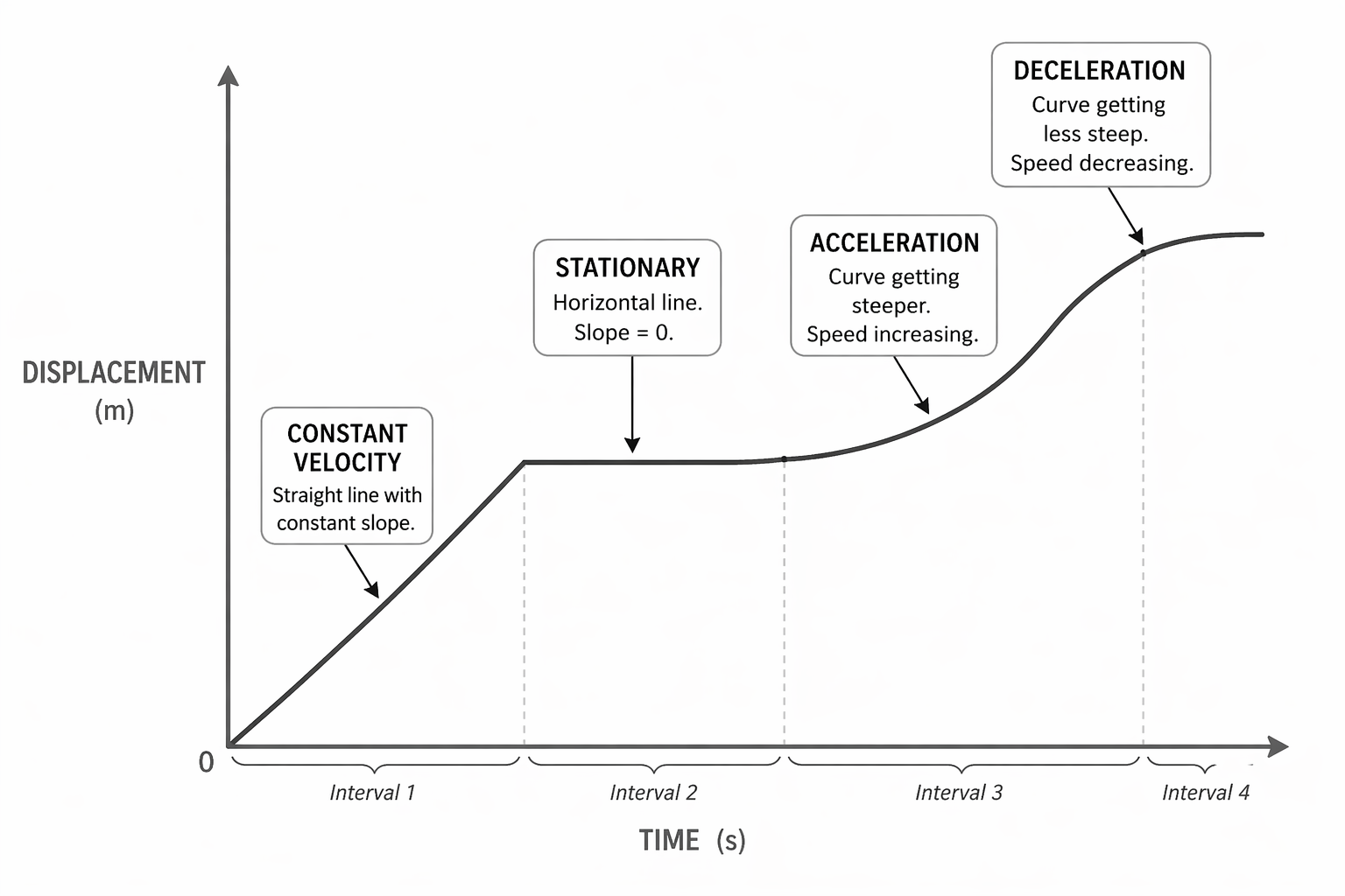
Figure: A displacement-time graph shows position changing with time; its gradient gives the velocity in 1D.

Velocity-Time Graph

Gradient gives acceleration (signed scalar):

$$\text{gradient}=\frac{dv}{dt}=a$$

Area under graph gives displacement (signed scalar):

$$\text{area}=\Delta s$$

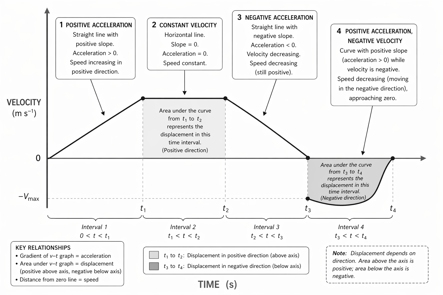
Figure: A velocity-time graph links kinematics directly: gradient gives acceleration and signed area under the graph gives displacement.

Acceleration-Time Graph

Area under graph gives change in velocity (signed scalar):

$$\text{area}=\Delta v$$

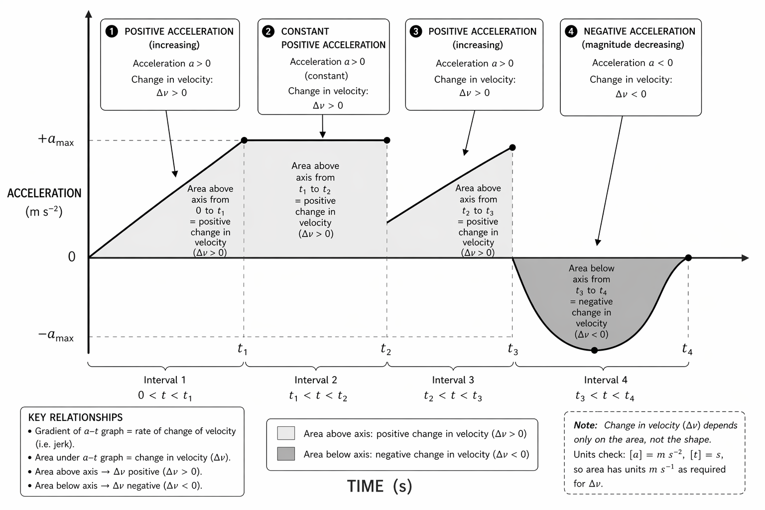
Figure: An acceleration-time graph shows how acceleration varies with time; the signed area under the graph gives the change in velocity.

Instantaneous Gradient

For curved graphs, draw a tangent.

Its gradient gives the instantaneous rate of change.

See Kinematics Graphs and Calculus

Constant Acceleration Models

When acceleration is constant in one dimension, use the SUVAT equations.

Variables:

• $s$ = displacement
• $u$ = initial velocity
• $v$ = final velocity
• $a$ = constant acceleration
• $t$ = time

SUVAT Equations

$$v=u+at$$ $$s=ut+\frac{1}{2}a{t}^2$$ $$v^2=u^2+2as$$ $$s=\frac{u+v}{2}t$$

Conditions for Using SUVAT

Use only when:

• motion is along one straight line (or one component)
• acceleration is constant
• same object throughout
• signs are consistent

Do not use directly when acceleration changes with time (e.g. varying air resistance).

See Constant Acceleration Models

Short Worked Examples

Example 1: Braking Car

A car travels at $u=20{\text{m s}}^{-1}$ and brakes uniformly at $a=-4.0{\text{m s}}^{-2}$.

Find stopping time.

Using:

$$v=u+at$$ $$0=20-4t$$ $$t=5.0\text{s}$$

Example 2: Falling Ball

Ball dropped from rest for $2.0\text{s}$, neglect air resistance.

Take downward positive.

$$u=0,a=g=9.81$$ $$s=ut+\frac{1}{2}a{t}^2$$ $$s=0+\frac{1}{2}(9.81)(2.0{)}^2=19.6\text{m}$$

Bridge to Projectile Motion

Kinematics ideas extend naturally to two dimensions.

A projectile is analysed by separating motion into (take right positive and upward positive):

Horizontal

$$a_x=0$$

Vertical

$$a_y=-g$$

The two motions share the same time.

This topic only introduces the idea. Full treatment:

Projectile Motion

Support page:

Projectile and Relative Motion

1D Motion Formula Summary

Rates

$$v=\frac{ds}{dt}$$ $$a=\frac{dv}{dt}$$

Graph Areas

$$\int vdt=\Delta s$$ $$\int adt=\Delta v$$

SUVAT

$$v=u+at$$ $$s=ut+\frac{1}{2}a{t}^2$$ $$v^2=u^2+2as$$ $$s=\frac{u+v}{2}t$$

Common Exam Pitfalls

• confusing distance with displacement
• confusing speed with velocity
• treating negative velocity as slowing down
• forgetting to define positive direction
• using SUVAT when acceleration is not constant
• reading graph height instead of gradient/area
• forgetting acceleration may be non-zero when velocity is zero
• mixing horizontal and vertical projectile components

Related Links

• Kinematic Quantities and Sign Conventions
• Kinematics Graphs and Calculus
• Constant Acceleration Models
• Projectile and Relative Motion
• Projectile Motion
• Forces
• Dynamics
• Circular Motion

Projectile Motion

Projectile motion is two-dimensional motion under gravity. The method is to resolve the initial velocity into horizontal and vertical components:

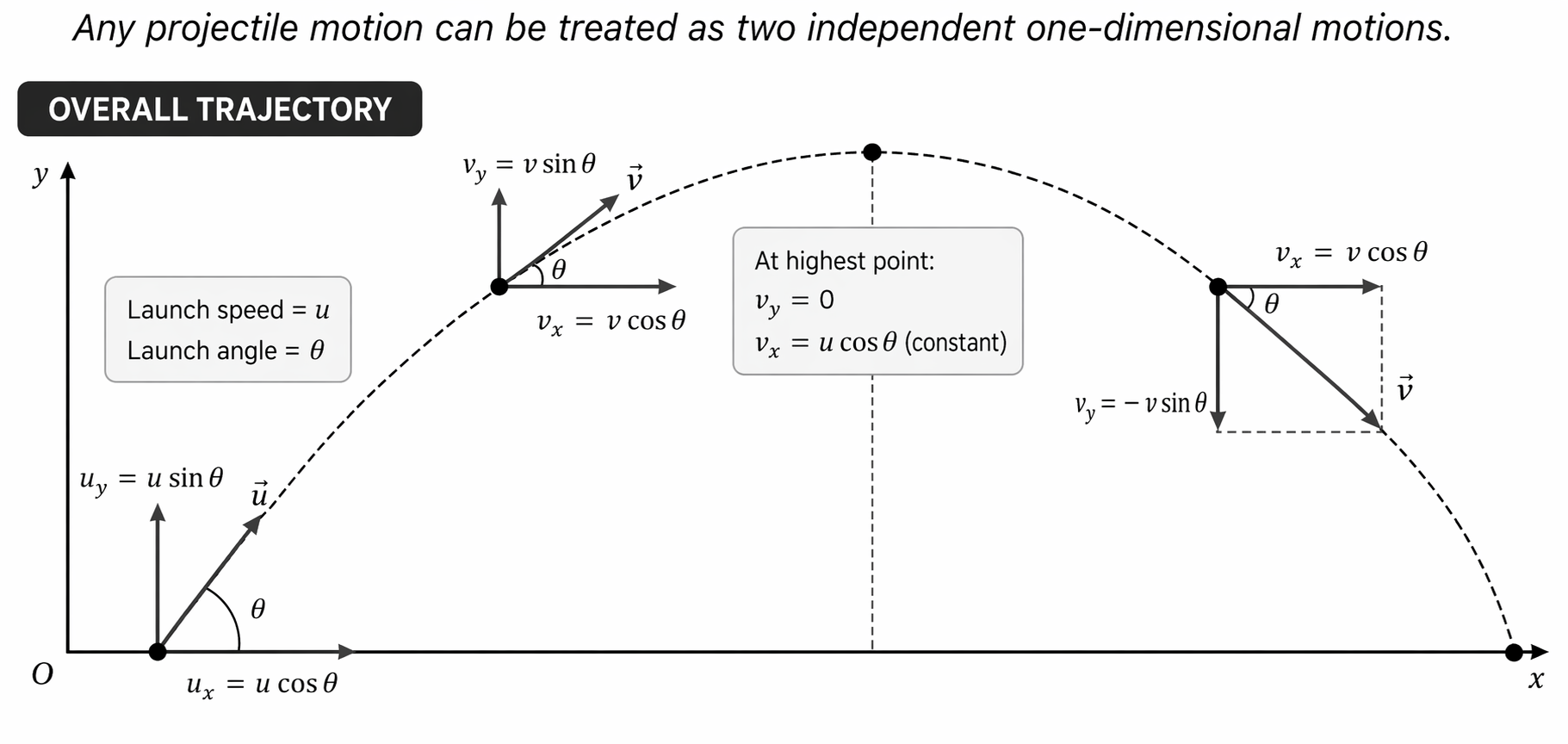$$ u_x=u\cos\theta $$ $$u_y=u\sin \theta$$

Then treat the two components separately:

$$a_x=0$$ $$a_y=-g$$

The horizontal and vertical motions are linked by the same time $t$. Do not mix horizontal displacement with vertical acceleration, or horizontal velocity with vertical velocity.

For fuller treatment, see Projectile Motion and Projectile and Relative Motion.

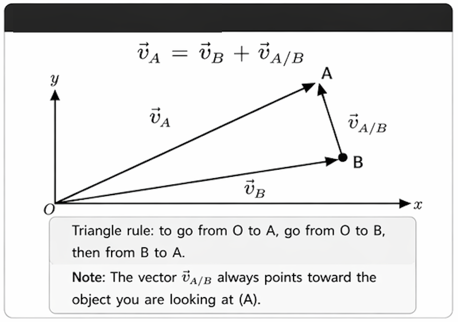
Relative Motion

Relative velocity describes how one object appears to move as seen from another object:

$${\vec{v}}_{A/B}={\vec{v}}_A-{\vec{v}}_B$$

This is useful when comparing two moving objects, such as a boat crossing a river, two cars moving along a road, or one projectile observed from another.

Learning Path

Use these deeper notes when more detail is needed:

• Kinematic Quantities and Sign Conventions
• Kinematics Graphs and Calculus
• Constant Acceleration Models
• Projectile Motion
• Projectile and Relative Motion

Exam Relevance

Kinematics is a foundational topic frequently tested in H2 Physics examinations, often integrated with dynamics and forces. Students are expected to apply the SUVAT equations correctly, paying close attention to sign conventions and model assumptions. Graphical analysis of motion, including interpreting gradients and areas, is crucial. Projectile motion problems require a systematic approach of resolving components and applying constant-acceleration equations independently to horizontal and vertical motion, using time as the linking variable. Understanding the conditions for speeding up or slowing down is also important for conceptual questions.

Common exam traps include:

• using SUVAT when acceleration is not constant;
• confusing distance with displacement or speed with velocity;
• treating negative velocity as automatically meaning slowing down;
• forgetting that displacement can be negative;
• reading graph height when the question asks for gradient or area;
• taking $g$ as positive or negative without first defining the sign convention;
• assuming acceleration is zero at the highest point of projectile motion;
• mixing horizontal and vertical components in projectile motion;
• forgetting that both projectile components share the same time.

Links

• Prerequisite: measurement
• Prerequisite: vectors
• Related: kinematic quantities and sign conventions
• Related: kinematics graphs and calculus
• Related: constant acceleration models
• Related: projectile motion
• Related: projectile and relative motion
• Related: dynamics
• Related: dynamics
• Related: work energy and power
• Related: circular motion
• Related: oscillations
• Related: electric fields
• Misconception: suvat applicability
• Misconception: sign convention errors
• Misconception: scalars vs vectors
• Misconception: negative acceleration always slowing down
• Misconception: projectile component mixing
• Misconception: projectile time link
• Misconception: projectile initial conditions

Provenance

• source file: 1_PDFsam_02_Kinematics.pdf
• generated by: bridging_tools/ingest_JC_phy_wiki.py
• manifest entry: inbox/lecture_notes/1_PDFsam_02_Kinematics.pdf
• source hash: e6bc8b67c3712cdf20e239e73e7594f52d142c51fffc795f23cae8984cda52d6